library(ggplot2)
library(bayesplot)
library(brms)
box::use(
  collapse[qsu]
)
options(brms.backend = "cmdstanr")
source("hhs-ggtheme.R")

# seed for R's pseudo-RNGs, not Stan's
set.seed(1123)Bayes Workshop Part 2
Intro
The first part of the tutorial contrasted the basics of Frequentist statistics with Bayesian statistics. We talked about what the practical advantages of each method are and why Bayesian statistics might be a useful tool for Accounting researchers. In part two we will illustrate how to fit Bayesian models. First we will cover some basic intuition behind MCMC, then we will fit some models to examine the role of team training to reduce internal control deficiency.
Conceptual understanding of fitting Bayesian models
Posterior distributions are difficult
Let’s say you have some data \(y\) and want to compute the posterior of some parameter \(\theta\) after seeing \(y\). This is difficult.
\[P(\theta \mid y)=\frac{P(y\mid\theta)P(\theta)}{P(y)}\]
As the bayesian updating formula illustrates, first we would need to multiply two probability density functions and then scaled it by another probability density function. The result is often analytically intractable. We cannot compute the resulting function in most cases. There are exceptions, combinations of likelihood and so-called conjugate priors, where the resulting form of the posterior is the same as the prior. Conjugate priors do not exist in every situation however, and they limit the range of possible priors to use. Hence, in modern statistics, we need to resort to sampling methods.
The idea behind MCMC
Sampling methods are an amazing and powerful innovation. They allow us to sample from any unknown distribution. It works well in the situation where we have a distribution \(P(z) = \frac{1}{Z_P}p(z)\), where it is easy to compute \(p(z)\) but hard to compute \(Z_P\). This is the case for \(P(\theta \mid y)=\frac{P(y\mid\theta)P(\theta)}{P(y)}\). We can often compute \(P(y\mid\theta)P(\theta)\) reasonably well. The problem is the scaler \(P(y)\), which is very difficult to compute (As it is technically the integral of \(P(y\mid\theta)\) over all possible values of \(\theta\)). However, if we set up the sampling method the right way, we can avoid having to compute \(P(y)\).
The simplest sampling method, the Metropolis Markov Chain Monte Carlo Sampler is a good way of explaining the intuition behind most sampling methods. Compared to more modern samplers Metropolis MCMC is quite inefficient. The tools we are going to use later use a sampler called Hamiltonian MCMC. We won’t really cover it here because we don’t have time. However, if you are seriously considering using Bayesian methods, you should familiarize yourself a bit with it. For complicated models, you might need to tune the sampler a bit and for that you need to understand how it works. A good starting resource (in general) are the incredibly good teaching materials by Richard McElreath on YouTube.
Back to Metropolis Hastings MCMC. The following is adapted from wikipedia: Let \(f(\theta)\) be a function that is proportional to the desired posterior probability density function \(P(\theta \mid y)\). We will repeat the following steps for \(n\) number of steps. And we call the series of \(n\) steps a chain.
- To begin: Choose an arbitrary point \(\theta_0\) to be the first “sample”. Choose an arbitrary probability density \(g( \theta_t \mid \theta_{t-1} )\). The requirement for this is a function that proposes new “candidates” for the next sample \(\theta_t\), given the previous sample value. A common choice is a Gaussian distribution centered at \(\theta_{t-1}\), so that points closer to \(\theta_{t-1}\) are more likely to be visited next, making the sequence of samples into a random walk. We call this the proposal density function (jumping function)
- For each iteration t (the \(n\) steps):
- Generate a candidate \(\theta_t'\) for the next sample using \(g( \theta_t \mid \theta_{t-1} )\).
- Calculate the acceptance ratio \({\displaystyle \alpha =f(\theta_t')/f(\theta_{t-1})}\), which will be used to decide whether to accept or reject the candidate.
- Generate a uniform random number \(u \in [ 0 , 1 ]\).
- If \(u\leq \alpha\), then accept the candidate by setting \(\theta_t = \theta_t'\), else reject the candidate and set \(\theta_t = \theta_{t-1}\).
Computing the acceptance ratio is how we avoid having to compute \(P(Y)\). Because \(f\) is essentially P(y)P(). Which means:
\[a = \frac{f(\theta_t')}{f(\theta_{t-1})} = \frac{P(y\mid\theta_t')P(\theta_t')}{P(y\mid\theta_{t-1})P(\theta_{t-1})}=\frac{P(\theta_t'\mid y)}{P(\theta_{t-1}\mid y)}\] This algorithm proceeds by randomly attempting to move about the sample space, sometimes accepting the moves and sometimes remaining in place. Note that the acceptance ratio \(\alpha\) indicates how probable the new proposed sample is with respect to the current sample, according to the posterior distribution. If we attempt to move to a point that is more probable than the existing point (i.e. a point in a higher-density region of \(P(\theta\mid y)\) corresponding to an \({\displaystyle \alpha >1\geq u})\), we will always accept the move.
Because we start at a random spot in parameter space, it might take some time for the chain to “find” the posterior distribution (loosely speaking). Often we run not one of these chains, but many (default is to use 4) to see whether they have converged to traversing the posterior region. To visualize how this all looks, here is an animation borrowed from this great post by Maxwell B. Joseph

The Case
For the rest of part two we will use the following made-up research case:
You want to examine whether team-level training of operating teams helps in reducing internal control deficiencies. Via a national research center, you managed to find firms willing to participate in a field experiment where you randomly assign and conduct team-level training with the help of an advisory firm. You do this for a few months and record the level of internal control deficiencies as reported by internal audits.
Our question of interest is thus whether team-training is effective at reducing internal control weakness. In addition, we also want to know additional characteristics of any potential team-training effect. Bayesian analysis is particularly suited for these type of questions and we’ll use this simple (and unfortunately unrealistic example) to illustrate how to perform Bayesian stats with R.
Setup
The data
dta <- readRDS('data/contrdef.rds')
str(dta)
'data.frame': 120 obs. of 9 variables:
$ firm_id : int 1 1 1 1 1 1 1 1 1 1 ...
$ quarter : int 1 2 3 4 5 6 7 8 9 10 ...
$ firm_size : num 21189 21189 21189 21189 21189 ...
$ firm_int : num -9.52 -9.52 -9.52 -9.52 -9.52 ...
$ firm_train: num 0.0864 0.0864 0.0864 0.0864 0.0864 ...
$ training : num 6 2 5 3 4 3 0 0 2 8 ...
$ noise : num 0.1363 0.0823 0.1308 0.1747 0.1745 ...
$ eta : num 0.962 0.617 0.876 0.703 0.789 ...
$ contrdef : num 1 1 5 2 2 0 1 2 3 0 ...We have access to the following important fields:
firm_id: The unique firm identifierquarter: The number of the quarter in which the training was conductedfirm_size: The amount of revenues in that quarter in T$training: How many trainings were conducted in that firm in that quartercontrdef: The count of internal control deficiencies found in a 90 day window after the end of the quarter
Descriptives of the data
c(
  "n firms" = length(unique(dta$firm_id)),
  "n quarters" = length(unique(dta$quarter))
)
n firms n quarters
10 12 qsu(dta) N Mean SD Min Max
firm_id 120 5.5 2.8843 1 10
quarter 120 6.5 3.4665 1 12
firm_size 120 87464.5 51260.4165 17902 166954
firm_int 120 -9.5598 0.0934 -9.7066 -9.3488
firm_train 120 -0.3374 0.3344 -0.984 0.1061
training 120 2.275 1.8469 0 8
noise 120 0.1058 0.0443 -0.0097 0.1889
eta 120 0.8819 1.2766 -3.5323 2.6158
contrdef 120 4.675 8.4894 0 49ggplot(dta, aes(x = contrdef)) +
geom_bar()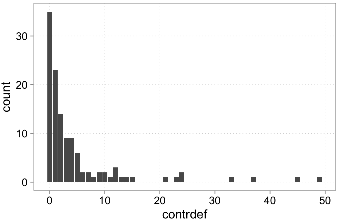
Modeling the data DGP
Starting point is our dependent variable
We have count data. That means we can think of various choices for processes generating count data. We can go with a normal distribution which basically means a normal linear regression. However, normal distributions are really more suitable for continuous data. We have count data—integer numbers that are distinct. One candidate distribution we could use to model the data generation is a Poisson distribution. We need to be careful here though. Poisson random variables have a special property: their variance equals the mean. Real-world count data very frequently has a variance that is higher than the mean. We call this ``over-dispersed’’ data. There are some ways to model this and we will use them. For didactic purposes we’ll start with poisson and test for over-dispersion.
The rest of the model
Given that we have chosen a Poisson regression as our main distribution, we define the likelihood as follows (For firm \(i = 1,\dots,10\) at time (quarter) \(t = 1,\dots,12\)):
\[ \begin{align*} \textrm{contrdef}_{i,t} & \sim \textrm{Poisson}(\lambda_{i,t}) \\ \lambda_{i,t} & = \exp{(\eta_{i,t})} \\ \eta_{i,t} &= b_0 + b_1 \, \textrm{training}_{i,t} \end{align*} \]
Fitting a simple Bayesian model
For more complicated models we prefer to code the model directly in the stan language and use cmdstanr to fit it. The models in this tutorial can all be fit using simple formulas and using the awesome brms package.
fit_simple <- brm(
  contrdef ~ 1 + training,
  family = poisson,
  data = dta,
  prior = c(
    prior("normal(0, 10)", class = "Intercept"),
    prior("normal(0, 10)", class = "b", coef = "training")
    ),
  chains = 4, cores = 4,
  refresh = 0
)
Fit summary
summary(fit_simple) Family: poisson
Links: mu = log
Formula: contrdef ~ 1 + training
Data: dta (Number of observations: 120)
Draws: 4 chains, each with iter = 2000; warmup = 1000; thin = 1;
total post-warmup draws = 4000
Population-Level Effects:
Estimate Est.Error l-95% CI u-95% CI Rhat Bulk_ESS Tail_ESS
Intercept 1.73 0.06 1.61 1.86 1.00 3403 2649
training -0.09 0.02 -0.14 -0.04 1.00 2678 2389
Draws were sampled using sample(hmc). For each parameter, Bulk_ESS
and Tail_ESS are effective sample size measures, and Rhat is the potential
scale reduction factor on split chains (at convergence, Rhat = 1).prior_summary(fit_simple)| prior | class | coef | group | resp | dpar | nlpar | lb | ub | source |
|---|---|---|---|---|---|---|---|---|---|
| b | default | ||||||||
| normal(0, 10) | b | training | user | ||||||
| normal(0, 10) | Intercept | user |
The summary statistics are based on the empirical histogram of the four markov chains we fit. Here is how they looked:
Checking the sampling
mcmc_hist(fit_simple, pars = c("b_Intercept", "b_training"))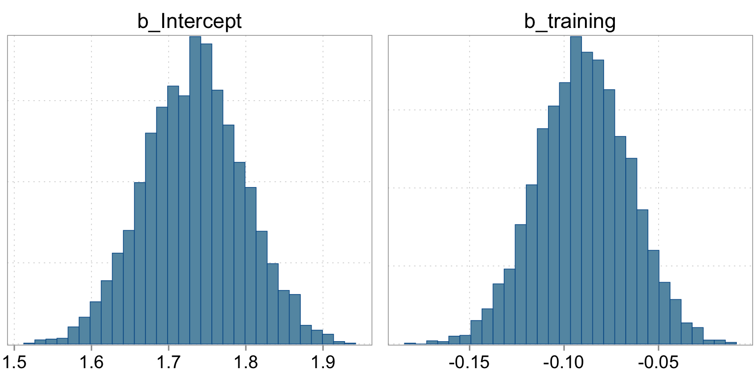
We should also have a quick look at the chains themselves:
bayesplot::mcmc_trace(fit_simple)
Checking the fit
Above we talked about the issue of over-dispersion. Let’s take a look at our model “fit” versus the actual data
y_pred <- posterior_predict(fit_simple)
ppc_dens_overlay(y = dta$contrdef, yrep = y_pred[1:200,])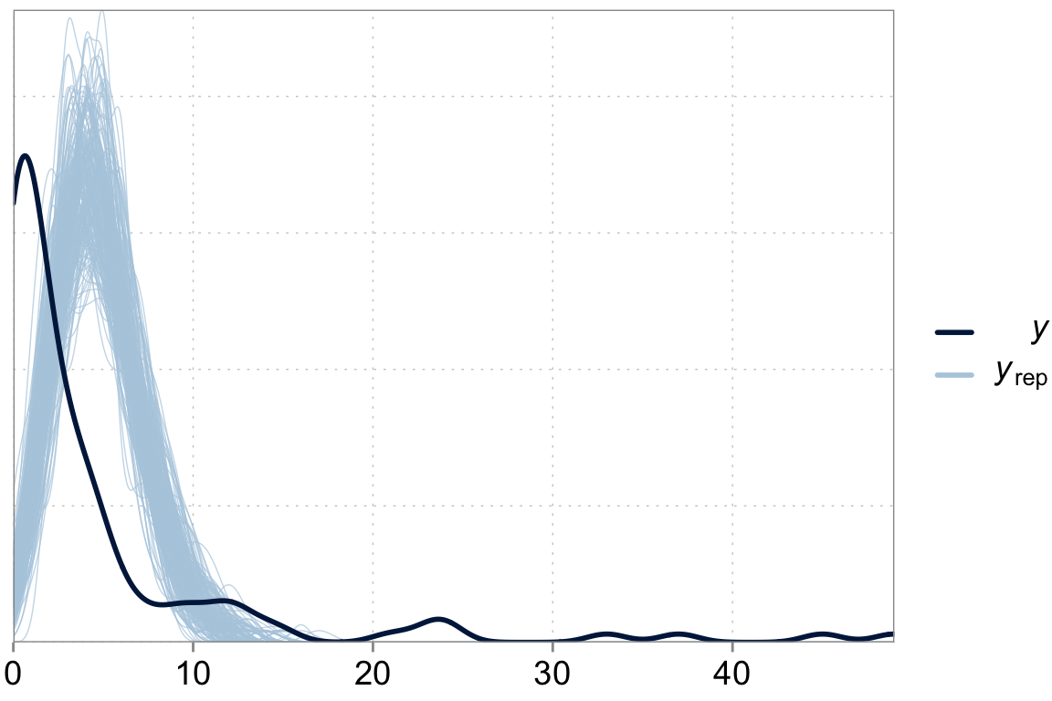
We are underpredicting zero counts, overpredicting middle range counts and maybe slightly underpredicting large counts. That looks like our poisson model with its property that the variance should equal the mean has issues fitting well. \(\lambda\), controls both the expected counts and the variance of these counts. We can fix that.
Modelling over-dispersion
A common DGP model for fitting overdispersed data is the negative-binomial distribution. We also add a two control variables.
\[ \begin{align*} \textrm{contrdef}_{i,t} & \sim \textrm{Neg-Binomial}(\lambda_{i,t}, \phi) \\ \lambda_{i,t} & = \exp{(\eta_{i,t})} \\ \eta_{i,t} &= b_0 + b_1 \,\textrm{training}_{i,t} + \textrm{log\_firm\_size}_{i} \end{align*} \]
To understand what is going on here, just note that the negative binomial pdf is parameterized in terms of its log-mean, \(\eta\), and it has a precision, \(\phi\), that affects it’s variance. The mean and variance of \(y = \textrm{contrdef}\) is thus:
\[ \mathbb{E}[y] \, = \lambda = \exp(\eta) \]
\[ \text{Var}[y] = \lambda + \lambda^2/\phi = \exp(\eta) + \exp(\eta)^2 / \phi. \]
As \(\phi\) gets larger the term \(\lambda^2 / \phi\) approaches zero and so the variance of the negative-binomial approaches \(\lambda\), i.e., the negative-binomial gets closer and closer to the Poisson.
We include \(\textrm{log\_firm\_size}_{i}\) as an exposure term (note, it does not have a coefficient in front). Our previous poisson model’s mean parameter is a rate of deficiencies in the next quarter (90 days). However, in a way the “deficiency process” also plays out over a firm’s size (bigger, more complex firms have more opportunities for deficiencies to occur). We have revenues in T$ as a measure of firm size. If we multiply \(\lambda\) by \(\textrm{firm\_size}_{i}\), we can interpret our coefficients as shifting a rate of deficiencies per T$ revenues per next 90 days. The last trick is to log firm size in order to put it into \(\eta\).
Fitting a negative binomial model
fit_negbin <- brm(
  contrdef ~ 1 + training + offset(log(firm_size)),
  family = negbinomial,
  data = dta,
  prior = c(
    prior("normal(0, 10)", class = "Intercept"),
    prior("normal(0, 10)", class = "b", coef = "training")
    ),
  chains = 4, cores = 4,
  refresh = 0
)
Fit summary
summary(fit_negbin) Family: negbinomial
Links: mu = log; shape = identity
Formula: contrdef ~ 1 + training + offset(log(firm_size))
Data: dta (Number of observations: 120)
Draws: 4 chains, each with iter = 2000; warmup = 1000; thin = 1;
total post-warmup draws = 4000
Population-Level Effects:
Estimate Est.Error l-95% CI u-95% CI Rhat Bulk_ESS Tail_ESS
Intercept -9.77 0.22 -10.18 -9.33 1.00 3588 2547
training 0.00 0.07 -0.14 0.14 1.00 3840 2733
Family Specific Parameters:
Estimate Est.Error l-95% CI u-95% CI Rhat Bulk_ESS Tail_ESS
shape 0.54 0.09 0.39 0.73 1.00 3370 2670
Draws were sampled using sample(hmc). For each parameter, Bulk_ESS
and Tail_ESS are effective sample size measures, and Rhat is the potential
scale reduction factor on split chains (at convergence, Rhat = 1).The coefficients have changed. Note that partly this is also because we are now looking at the rate of deficiencies per 90 days per T$ in revenues
prior_summary(fit_negbin)| prior | class | coef | group | resp | dpar | nlpar | lb | ub | source |
|---|---|---|---|---|---|---|---|---|---|
| b | default | ||||||||
| normal(0, 10) | b | training | user | ||||||
| normal(0, 10) | Intercept | user | |||||||
| gamma(0.01, 0.01) | shape | 0 | default |
Checking the sampling
mcmc_hist(fit_negbin, pars = c("b_Intercept", "b_training", "shape"))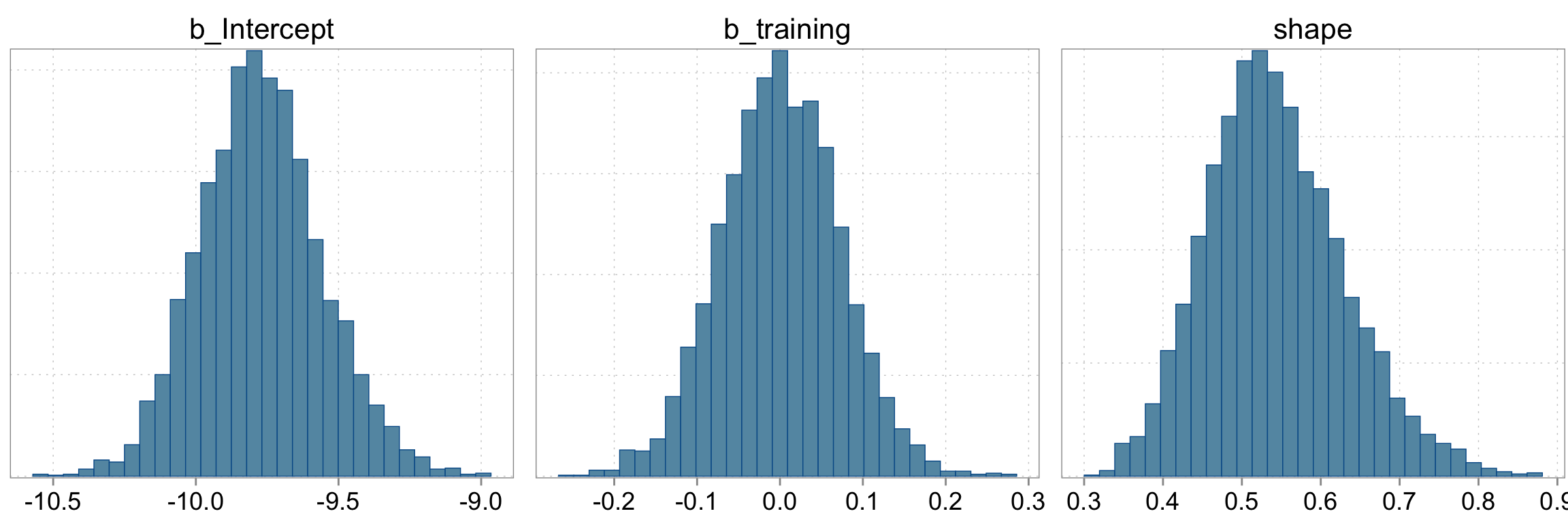
We should also have a quick look at the chains themselves:
bayesplot::mcmc_trace(fit_negbin)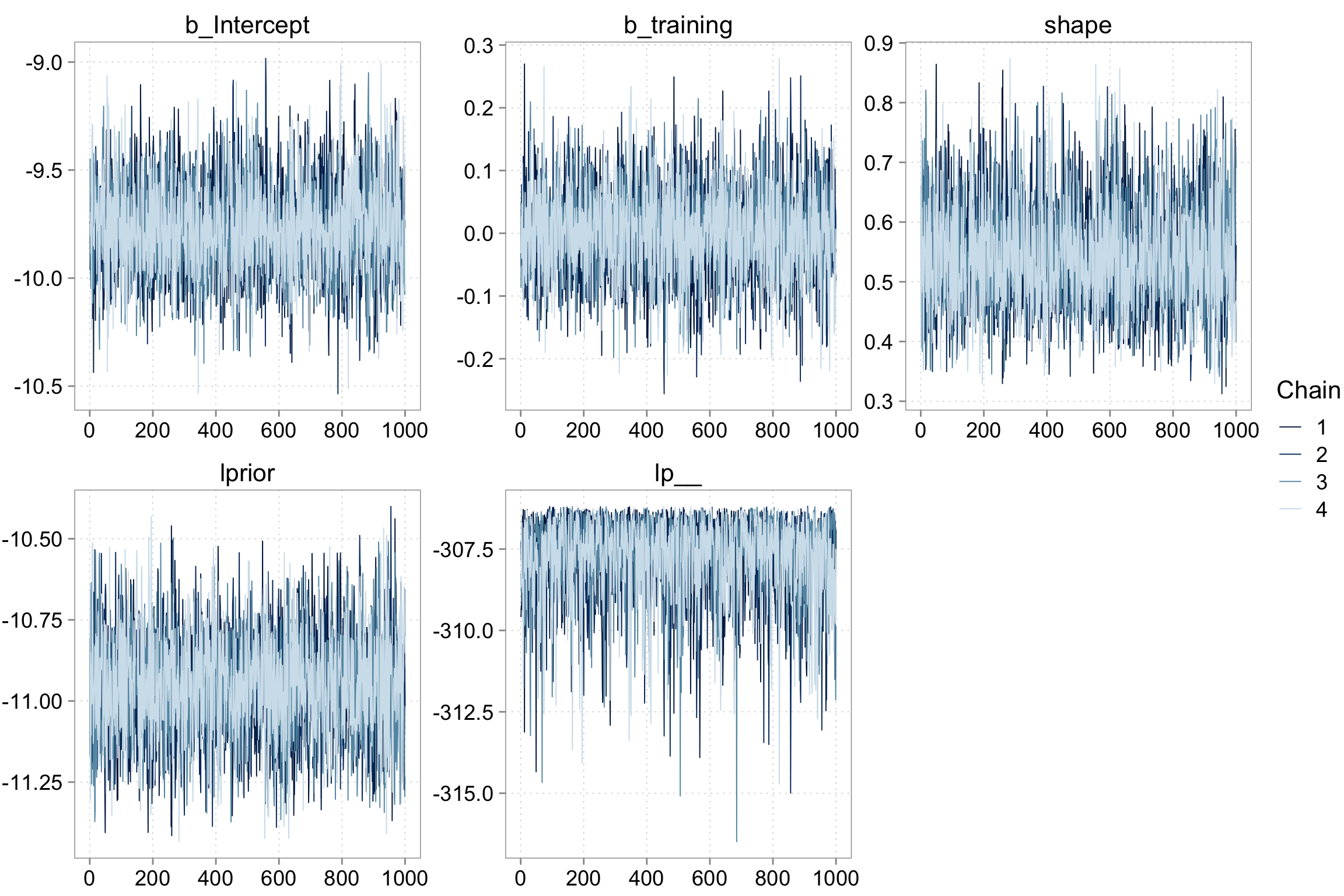
Checking the model fit
Above we talked about the issue of over-dispersion. Let’s take a look at our model “fit” versus the actual data
y_pred2 <- posterior_predict(fit_negbin)
ppc_dens_overlay(y = dta$contrdef, yrep = y_pred2[1:200,])
This looks like a much better fit.
The power of Bayes: Multilevel models
We are not necessarily done here. We purposefully framed the question as a field experiment, so that we do not have to worry about confounding issues. Training is basically randomized. We can still try to get a more precise estimate. And we can also see if there is meaningful variation in the effectiveness of training across firms. Especially the last question is something that multilevel models employing priors can really help with.
We will first built a model that only includes firm-specific intercepts. Afterwards we’ll add firm-specific slopes for \(training\) as well.
Fitting a varying intercepts model
fit_varint <- brm(
  contrdef ~ 1 + training + offset(log(firm_size)) + (1 | firm_id),
  family = negbinomial,
  data = dta,
  prior = c(
    prior("normal(0, 10)", class = "Intercept"),
    prior("normal(0, 10)", class = "b", coef = "training"),
    prior("normal(0, 1)", class = "sd", coef = "Intercept", group = "firm_id")
    ),
  chains = 4, cores = 4,
  refresh = 0
)
Fit summary
summary(fit_varint) Family: negbinomial
Links: mu = log; shape = identity
Formula: contrdef ~ 1 + training + offset(log(firm_size)) + (1 | firm_id)
Data: dta (Number of observations: 120)
Draws: 4 chains, each with iter = 2000; warmup = 1000; thin = 1;
total post-warmup draws = 4000
Group-Level Effects:
~firm_id (Number of levels: 10)
Estimate Est.Error l-95% CI u-95% CI Rhat Bulk_ESS Tail_ESS
sd(Intercept) 0.90 0.26 0.50 1.51 1.00 1086 1870
Population-Level Effects:
Estimate Est.Error l-95% CI u-95% CI Rhat Bulk_ESS Tail_ESS
Intercept -9.60 0.37 -10.33 -8.88 1.00 1379 1866
training -0.20 0.08 -0.34 -0.05 1.00 3333 3113
Family Specific Parameters:
Estimate Est.Error l-95% CI u-95% CI Rhat Bulk_ESS Tail_ESS
shape 0.81 0.15 0.56 1.14 1.00 3631 2712
Draws were sampled using sample(hmc). For each parameter, Bulk_ESS
and Tail_ESS are effective sample size measures, and Rhat is the potential
scale reduction factor on split chains (at convergence, Rhat = 1).There is some variation explained by varying intercepts. But it does not seem like it’s doing much in terms of improving the model fit.
prior_summary(fit_varint)| prior | class | coef | group | resp | dpar | nlpar | lb | ub | source |
|---|---|---|---|---|---|---|---|---|---|
| b | default | ||||||||
| normal(0, 10) | b | training | user | ||||||
| normal(0, 10) | Intercept | user | |||||||
| student_t(3, 0, 2.5) | sd | 0 | default | ||||||
| sd | firm_id | default | |||||||
| normal(0, 1) | sd | Intercept | firm_id | user | |||||
| gamma(0.01, 0.01) | shape | 0 | default |
The summary statistics are based on the empirical histogram of the four markov chains we fit. Here is how they looked:
Checking the sampling
parnames(fit_varint)Warning: 'parnames' is deprecated. Please use 'variables' instead. [1] "b_Intercept" "b_training"
[3] "sd_firm_id__Intercept" "shape"
[5] "r_firm_id[1,Intercept]" "r_firm_id[2,Intercept]"
[7] "r_firm_id[3,Intercept]" "r_firm_id[4,Intercept]"
[9] "r_firm_id[5,Intercept]" "r_firm_id[6,Intercept]"
[11] "r_firm_id[7,Intercept]" "r_firm_id[8,Intercept]"
[13] "r_firm_id[9,Intercept]" "r_firm_id[10,Intercept]"
[15] "lprior" "lp__" mcmc_hist(fit_varint)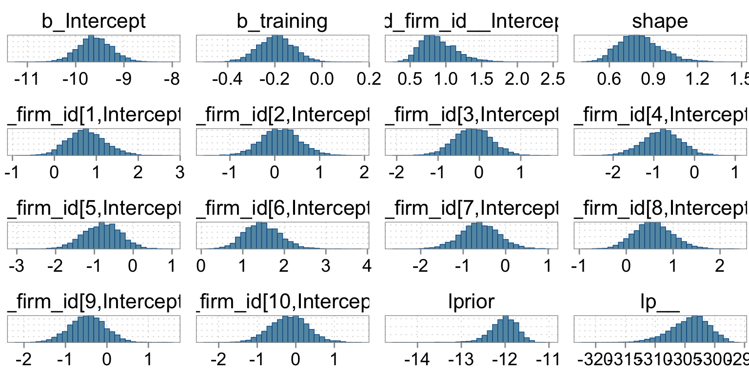
We should also have a quick look at the chains themselves:
bayesplot::mcmc_trace(
  fit_varint,
  pars = c("b_Intercept", "b_training", "shape", "sd_firm_id__Intercept")
  )
Checking the fit
Above we talked about the issue of over-dispersion. Let’s take a look at our model “fit” versus the actual data
y_pred <- posterior_predict(fit_varint)
ppc_dens_overlay(y = dta$contrdef, yrep = y_pred[1:200,])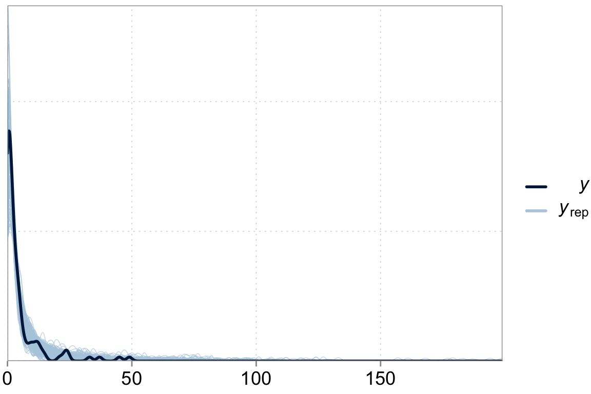
Fitting a varying intercepts varying slopes model
fit_varslopes <- brm(
  contrdef ~ 1 + training + offset(log(firm_size)) + (1 + training| firm_id),
  family = negbinomial,
  data = dta,
  prior = c(
    prior("normal(0, 10)", class = "Intercept"),
    prior("normal(0, 10)", class = "b", coef = "training"),
    prior("normal(0, 1)", class = "sd", coef = "Intercept", group = "firm_id"),
    prior(lkj(2), class = "cor")
    ),
  chains = 4, cores = 4,
  refresh = 0
)
Fit summary
summary(fit_varslopes)Warning: There were 1 divergent transitions after warmup. Increasing
adapt_delta above 0.8 may help. See
http://mc-stan.org/misc/warnings.html#divergent-transitions-after-warmup Family: negbinomial
Links: mu = log; shape = identity
Formula: contrdef ~ 1 + training + offset(log(firm_size)) + (1 + training | firm_id)
Data: dta (Number of observations: 120)
Draws: 4 chains, each with iter = 2000; warmup = 1000; thin = 1;
total post-warmup draws = 4000
Group-Level Effects:
~firm_id (Number of levels: 10)
Estimate Est.Error l-95% CI u-95% CI Rhat Bulk_ESS
sd(Intercept) 0.26 0.20 0.01 0.74 1.00 2018
sd(training) 0.44 0.15 0.22 0.81 1.00 980
cor(Intercept,training) -0.07 0.43 -0.83 0.77 1.00 576
Tail_ESS
sd(Intercept) 1599
sd(training) 2002
cor(Intercept,training) 1236
Population-Level Effects:
Estimate Est.Error l-95% CI u-95% CI Rhat Bulk_ESS Tail_ESS
Intercept -9.69 0.20 -10.06 -9.28 1.00 3357 3136
training -0.26 0.16 -0.61 0.04 1.00 1449 1623
Family Specific Parameters:
Estimate Est.Error l-95% CI u-95% CI Rhat Bulk_ESS Tail_ESS
shape 1.06 0.21 0.70 1.53 1.00 4304 2996
Draws were sampled using sample(hmc). For each parameter, Bulk_ESS
and Tail_ESS are effective sample size measures, and Rhat is the potential
scale reduction factor on split chains (at convergence, Rhat = 1).prior_summary(fit_varslopes)| prior | class | coef | group | resp | dpar | nlpar | lb | ub | source |
|---|---|---|---|---|---|---|---|---|---|
| b | default | ||||||||
| normal(0, 10) | b | training | user | ||||||
| normal(0, 10) | Intercept | user | |||||||
| lkj_corr_cholesky(2) | L | user | |||||||
| L | firm_id | default | |||||||
| student_t(3, 0, 2.5) | sd | 0 | default | ||||||
| sd | firm_id | default | |||||||
| normal(0, 1) | sd | Intercept | firm_id | user | |||||
| sd | training | firm_id | default | ||||||
| gamma(0.01, 0.01) | shape | 0 | default |
The summary statistics are based on the empirical histogram of the four markov chains we fit. Here is how they looked:
Visualizing varying slopes
parnames(fit_varslopes)Warning: 'parnames' is deprecated. Please use 'variables' instead. [1] "b_Intercept" "b_training"
[3] "sd_firm_id__Intercept" "sd_firm_id__training"
[5] "cor_firm_id__Intercept__training" "shape"
[7] "r_firm_id[1,Intercept]" "r_firm_id[2,Intercept]"
[9] "r_firm_id[3,Intercept]" "r_firm_id[4,Intercept]"
[11] "r_firm_id[5,Intercept]" "r_firm_id[6,Intercept]"
[13] "r_firm_id[7,Intercept]" "r_firm_id[8,Intercept]"
[15] "r_firm_id[9,Intercept]" "r_firm_id[10,Intercept]"
[17] "r_firm_id[1,training]" "r_firm_id[2,training]"
[19] "r_firm_id[3,training]" "r_firm_id[4,training]"
[21] "r_firm_id[5,training]" "r_firm_id[6,training]"
[23] "r_firm_id[7,training]" "r_firm_id[8,training]"
[25] "r_firm_id[9,training]" "r_firm_id[10,training]"
[27] "lprior" "lp__" mcmc_areas(fit_varslopes,
pars = paste0("r_firm_id[", 1:10,",training]"),
prob = 0.95)
Checking the sampling
mcmc_hist(
  fit_varslopes,
  pars = c("b_Intercept", "b_training", "shape", "sd_firm_id__Intercept",
           "cor_firm_id__Intercept__training", "sd_firm_id__training")
  )
We should also have a quick look at the chains themselves:
bayesplot::mcmc_trace(
  fit_varslopes,
  pars = c("b_Intercept", "b_training", "shape", "sd_firm_id__Intercept",
           "cor_firm_id__Intercept__training", "sd_firm_id__training")
  )
Checking the fit
Above we talked about the issue of over-dispersion. Let’s take a look at our model “fit” versus the actual data
y_pred <- posterior_predict(fit_varslopes)
ppc_dens_overlay(y = dta$contrdef, yrep = y_pred[1:200,])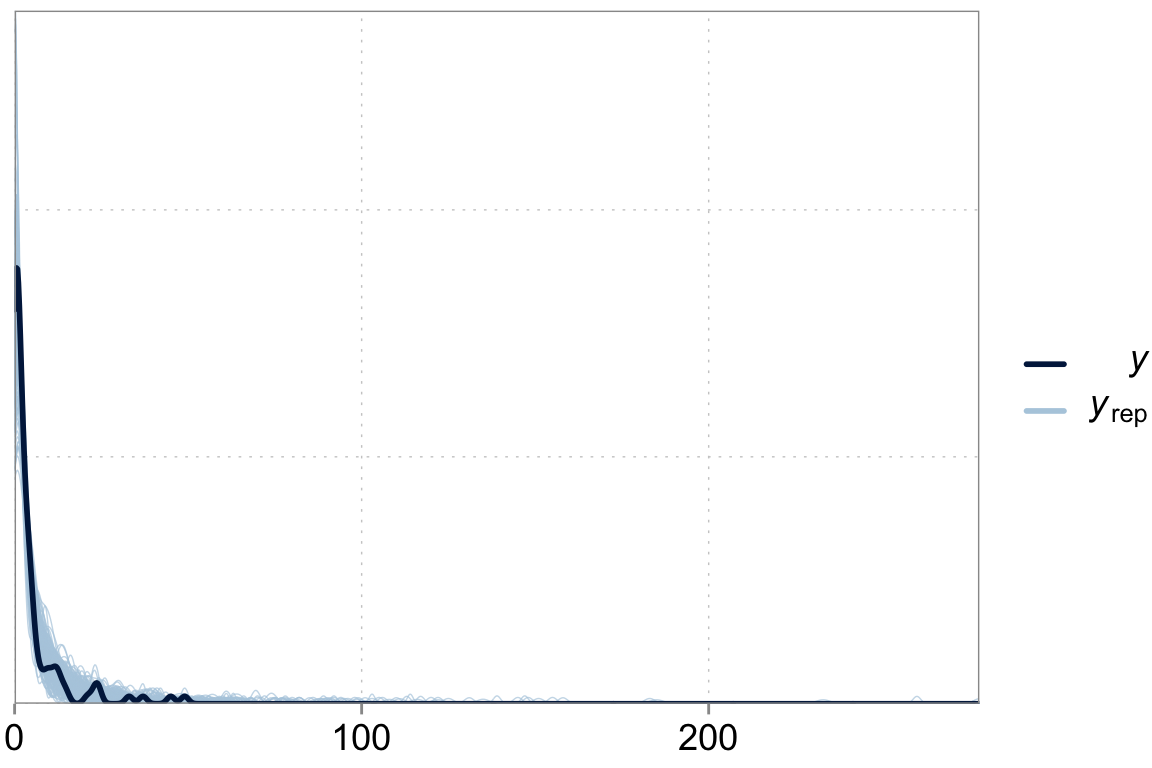
Model comparison
fit_simple <- add_criterion(fit_simple, "loo")Warning: Found 2 observations with a pareto_k > 0.7 in model 'fit_simple'. It
is recommended to set 'moment_match = TRUE' in order to perform moment matching
for problematic observations.fit_negbin <- add_criterion(fit_negbin, "loo")Warning: Found 1 observations with a pareto_k > 0.7 in model 'fit_negbin'. It
is recommended to set 'moment_match = TRUE' in order to perform moment matching
for problematic observations.fit_varint <- add_criterion(fit_varint, "loo")Warning: Found 1 observations with a pareto_k > 0.7 in model 'fit_varint'. It
is recommended to set 'moment_match = TRUE' in order to perform moment matching
for problematic observations.fit_varslopes <- add_criterion(fit_varslopes, "loo")Warning: Found 1 observations with a pareto_k > 0.7 in model 'fit_varslopes'.
It is recommended to set 'moment_match = TRUE' in order to perform moment
matching for problematic observations.loo_compare(fit_simple, fit_negbin, fit_varint, fit_varslopes) elpd_diff se_diff
fit_varslopes 0.0 0.0
fit_varint -9.6 5.1
fit_negbin -24.8 7.9
fit_simple -431.3 118.3