Fixed effects and Bayesian Multi-level models

Published

October 30, 2021

This is one of those posts I made mainly so that I have something to link to whenever I get this particular question.

The punchline

Consider a model with unobserved heterogeneity $a_{i}$ :

$y_{i, t} = a_{i} + a_{1} * x_{i, t} + u_{i, t}, c o v (a_{i}, x_{i, t}) \neq 0$

$a_{i}$ is meant to denote unobservable subject-specific heterogeneity that is confounding the relation of interest between $y$ and $x$ (because $c o v (a_{i}, x_{i, t}) \neq 0$ ). Fixed effects models, as commonly used in econometrics, remove between-subject variation to estimate the coefficient of interest ( $a_{1}$ ) using only within-variation. In the remainder of this short note, I assume that readers are similar with these type of fixed effects models.

Bayesian multi-level models can also account for $a_{i}$ , but one needs to consider that Bayesian multi-level models partially pool. Meaning, if one does not explicitly tell the model that there is a correlation between $a_{i}$ and $x_{i, t}$ , then it will partially pool the confounded between-variation and the within-variation. Incorporating this correlation is easy to do however. This note shows how.

Setup

library(cmdstanr)  # for fitting Bayesian models 
library(fixest)  # Fitting fixed effects models

Simulated data

For illustration purposes I simulate data from the following data generating process:

$a_{i} \sim N (2, 4)$

$x_{i, t} \sim 1.4 * a_{i} + N (0, 4)$

$y_{i, t} \sim a_{i} + 1 * x_{i, t} + N (0, 4)$

So, the true value of $a_{1}$ will be one in this simulation.

set.seed(753)

n_firms <- 100
periods <- 7

firm_id <- rep(1:n_firms, each = periods)
firm_mean <- rnorm(n_firms, 2, 4)
d <- data.frame(
  firm_id = firm_id,
  period = rep(1:periods, times = n_firms),
  firm_mean = rep(firm_mean, each = periods)
  )
# x is a function of the firm mean unobserved firm means
d$x <- rnorm(n_firms * periods, 0, 4) + 1.4 * d$firm_mean
# true coefficient of interest on x is 1
d$y <- d$firm_mean + 1 * d$x + rnorm(n_firms * periods, 0, 4)

# data container for bayesmodel
input_data <- list(
  N = nrow(d),
  J = max(d$firm_id),
  GroupID = d$firm_id,
  y = d$y,
  x = d$x,
  xm = 
    aggregate(
      cbind(x) ~ firm_id,
      data = d,
      FUN = \(h) c(mean = mean(h))
    )$x
)

Confounded pooled OLS estimate

Unsurprising, normal OLS will yield biased estimates because $c o v (a_{i}, x_{i, t}) \neq 0$ :

summary(lm(y ~ x, data = d))$coefficients

             Estimate Std. Error   t value      Pr(>|t|)
(Intercept) 0.6940142 0.19296977  3.596492  3.452875e-04
x           1.4855348 0.02437638 60.941562 1.120002e-281

Fixed effect estimate

For comparison purposes with the Bayesian models, here are the estimates of standard fixed effects models:

Using the fixestpackage:

olsfe <- feols(y ~ x | firm_id, data = d)
summary(olsfe)

OLS estimation, Dep. Var.: y
Observations: 700 
Fixed-effects: firm_id: 100
Standard-errors: Clustered (firm_id) 
  Estimate Std. Error t value  Pr(>|t|)    
x  1.02745   0.044027 23.3367 < 2.2e-16 ***
---
Signif. codes:  0 '***' 0.001 '**' 0.01 '*' 0.05 '.' 0.1 ' ' 1
RMSE: 3.75528     Adj. R2: 0.878907
                Within R2: 0.534057

The above fixed effects models yield estimates of 1.027, close to the true value of $a_{1} = 1$ . Just as expected.

Simple Bayesian multi-level model

In contrast to fixed effects models, which throw away between-subject-variation, Bayesian multi-level models model $a_{i}$ directly. In addition, these models have the advantage of applying adaptive shrinkage via partial pooling. This results in more stable and robust estimates of $a_{i}$ .

The model below does partial pooling by assuming that the $a_{i}$ follow a common distribution.

$a_{i} = μ_{a} + N (0, σ_{a})$

But it does not consider that $a_{i}$ and $x_{i, t}$ might be correlated. As a result the coefficient on x will be the partially pooled average of the between- and within-subject variation:

baymod_nocorr <- "
data{
  int<lower=1> N;                   // num obs
  int<lower=1> J;                   // num groups
  int<lower=1, upper=J> GroupID[N]; // GroupID for obs, e.g. FirmID or Industry-YearID
  vector[N] y;                      // Response
  vector[N] x;                      // Predictor
}
parameters{
  vector[J] z;                     // standard normal sampler
  real mu_a;                       // hypprior mean coefficients
  real<lower=0> sig_u;             // error-term scale
  real<lower=0> sig_a;             // error-term scale
  real a1;
}
transformed parameters{
  vector[J] ai;                     // intercept vector
  ai = mu_a + z * sig_a;
}
model{
  z ~ normal(0, 1);
  mu_a  ~ normal(0, 10);
  sig_u ~ exponential(1.0 / 8);
  sig_a ~ exponential(1.0 / 4);
  a1 ~ normal(0, 10);
  y ~ normal(ai[GroupID] + a1 * x, sig_u);
}
"
stanmod_nocorr <- cmdstan_model(write_stan_file(baymod_nocorr))

bayfit_nocorr <- stanmod_nocorr$sample(
  data = input_data,
  iter_sampling = 1000,
  iter_warmup = 1000,
  chains = 4,
  parallel_chains = 4,
  seed = 1234,
  refresh = 0
)

Running MCMC with 4 parallel chains...

Chain 1 finished in 0.7 seconds.
Chain 2 finished in 0.7 seconds.
Chain 3 finished in 0.7 seconds.
Chain 4 finished in 0.8 seconds.

All 4 chains finished successfully.
Mean chain execution time: 0.7 seconds.
Total execution time: 0.9 seconds.

bayfit_nocorr$summary(variables = c("a1", "mu_a", "sig_a", "sig_u"))

# A tibble: 4 × 10
  variable  mean median     sd    mad    q5   q95  rhat ess_bulk ess_tail
  <chr>    <num>  <num>  <num>  <num> <num> <num> <num>    <num>    <num>
1 a1        1.32   1.32 0.0499 0.0500 1.24   1.40  1.00     765.    1330.
2 mu_a      1.24   1.23 0.319  0.315  0.730  1.77  1.00    1243.    2228.
3 sig_a     2.25   2.26 0.399  0.403  1.60   2.90  1.00     658.     902.
4 sig_u     4.25   4.25 0.137  0.138  4.04   4.48  1.00    1528.    2219.

Here is a visual presentation of the posterior of $a_{1}$

bayesplot::mcmc_areas(bayfit_nocorr$draws("a1")) + ggplot2::xlim(0, 2)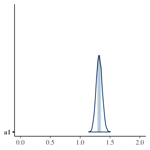

Bayesian multi-level model explicitely modelling correlation x and ai

This model gets rid of the problem, simply by explicitly modelling the correlation between $a_{i}$ and between-firm variation in $x_{i, t}$ as:

$a_{i} = μ_{a} + b * {\bar{x}}_{i} + N (0, σ_{a})$ $b$ will be the estimate of the between association, while $a 1$ estimates the within-variation. We still get shrinkage of $a_{i}$ around the between variation.

baymod_corr <- "
data{
  int<lower=1> N;                   // num obs
  int<lower=1> J;                   // num groups
  int<lower=1, upper=J> GroupID[N]; // GroupID for obs, e.g. FirmID or Industry-YearID
  vector[N] y;                      // Response
  vector[N] x;                      // Predictor
  vector[J] xm;                     // mean of x for groupID
}
parameters{
  vector[J] z;                     // standard normal sampler
  real mu_a;                       // hypprior mean coefficients
  real<lower=0> sig_u;             // error-term scale
  real<lower=0> sig_a;             // error-term scale
  real a1;
  real b;
}
transformed parameters{
  vector[J] ai;                     // intercept vector
  ai = mu_a + b * xm + z * sig_a;
}
model{
  z ~ normal(0, 1);
  mu_a  ~ normal(0, 10);
  sig_u ~ exponential(1.0 / 8);
  sig_a ~ exponential(1.0 / 8);
  a1 ~ normal(0, 10);
  b ~ normal(0, 10);
  y ~ normal(ai[GroupID] + a1 * x, sig_u);
}
"
stanmod_corr <- cmdstan_model(write_stan_file(baymod_corr))

bayfit_corr <- stanmod_corr$sample(
  data = input_data,
  iter_sampling = 1000,
  iter_warmup = 1000,
  chains = 4,
  parallel_chains = 4,
  seed = 123334,
  refresh = 0
)

Running MCMC with 4 parallel chains...

Chain 4 finished in 1.1 seconds.
Chain 2 finished in 1.1 seconds.
Chain 1 finished in 1.2 seconds.
Chain 3 finished in 1.2 seconds.

All 4 chains finished successfully.
Mean chain execution time: 1.1 seconds.
Total execution time: 1.3 seconds.

bayfit_corr$summary(variables = c("a1", "b", "mu_a", "sig_a", "sig_u"))

# A tibble: 5 × 10
  variable   mean median     sd    mad      q5   q95  rhat ess_bulk ess_tail
  <chr>     <num>  <num>  <num>  <num>   <num> <num> <num>    <num>    <num>
1 a1       1.03   1.03   0.0398 0.0392  0.961  1.09   1.00    3064.    2765.
2 b        0.652  0.652  0.0490 0.0490  0.572  0.732  1.00    3228.    2923.
3 mu_a     0.0616 0.0622 0.191  0.188  -0.251  0.375  1.00    3717.    2651.
4 sig_a    0.631  0.644  0.311  0.332   0.0939 1.13   1.00     749.    1487.
5 sig_u    4.08   4.07   0.119  0.118   3.88   4.27   1.00    3050.    2722.

$a 1$ is now centered on the true value.

bayesplot::mcmc_areas(bayfit_corr$draws("a1")) + ggplot2::xlim(0, 2)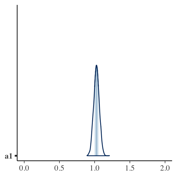

Another way of encoding the correlation between ai and x

The next piece of code more closely resembles the causal flow as I envision it. It encodes ${\bar{x}}_{i} \sim b 0 + b 1 * a_{i} + e_{x, i}$ . It fully recovers the simulation above (see the estimates of sig_a). The divergent transitions suggest that this model is harder to fit well. Not sure why that is. Something to figure out another day.

baymod_corr2 <- "
data{
  int<lower=1> N;                   // num obs
  int<lower=1> J;                   // num groups
  int<lower=1, upper=J> GroupID[N]; // GroupID for obs, e.g. FirmID or Industry-YearID
  vector[N] y;                      // Response
  vector[N] x;                      // Predictor
  vector[J] xm;                     // mean of x for groupID
}
parameters{
  vector[J] z;                     // standard normal sampler
  real mu_a;                       // hypprior mean coefficients
  real<lower=0> sig_u;             // error-term scale
  real<lower=0> sig_a;             // error-term scale
  real<lower=0> sig_x;             // error-term scale
  real a1;
  real b1;
  real b0;
}
transformed parameters{
  vector[J] ai;                     // intercept vector
  ai = mu_a + z * sig_a;
}
model{
  z ~ normal(0, 1);
  mu_a  ~ normal(0, 10);
  sig_u ~ exponential(1.0 / 8);
  sig_a ~ exponential(1.0 / 8);
  a1 ~ normal(0, 10);
  b1 ~ normal(0, 10);
  b0 ~ normal(0, 10);
  sig_x ~ exponential(1.0 / 7);
  xm ~ normal(b0 + b1 * ai, sig_x);
  y ~ normal(ai[GroupID] + a1 * x, sig_u);
}
"
stanmod_corr2 <- cmdstan_model(write_stan_file(baymod_corr2))

bayfit_corr2 <- stanmod_corr2$sample(
  data = input_data,
  iter_sampling = 1000,
  iter_warmup = 1000,
  adapt_delta = 0.9,
  chains = 4,
  parallel_chains = 4,
  seed = 123244,
  refresh = 0
)

Running MCMC with 4 parallel chains...

Chain 2 finished in 1.3 seconds.
Chain 1 finished in 1.4 seconds.
Chain 4 finished in 1.8 seconds.
Chain 3 finished in 2.0 seconds.

All 4 chains finished successfully.
Mean chain execution time: 1.6 seconds.
Total execution time: 2.0 seconds.

bayfit_corr2$summary(variables = c("a1", "b0", "b1", "mu_a", "sig_a", "sig_u", "sig_x"))

# A tibble: 7 × 10
  variable    mean  median     sd    mad     q5   q95  rhat ess_bulk ess_tail
  <chr>      <num>   <num>  <num>  <num>  <num> <num> <num>    <num>    <num>
1 a1       1.03    1.03    0.0395 0.0399  0.968 1.10   1.00    1068.    1501.
2 b0       0.00162 0.00387 0.296  0.286  -0.481 0.496  1.01    1381.    1993.
3 b1       1.52    1.51    0.119  0.120   1.34  1.72   1.00     682.     523.
4 mu_a     2.17    2.15    0.445  0.464   1.45  2.91   1.04     134.     444.
5 sig_a    3.97    3.96    0.399  0.398   3.36  4.66   1.01     333.     661.
6 sig_u    4.07    4.07    0.113  0.115   3.88  4.26   1.01    1188.    1738.
7 sig_x    1.08    1.08    0.368  0.398   0.507 1.70   1.06     119.     168.

bayesplot::mcmc_areas(bayfit_corr2$draws("a1")) + ggplot2::xlim(0, 2)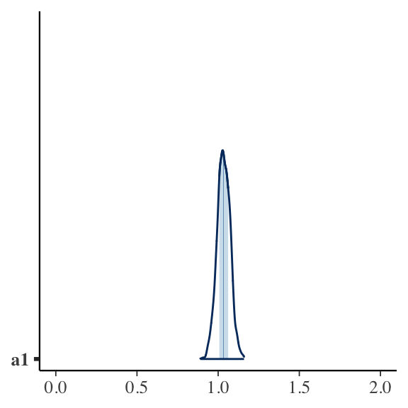

Why bother with a Bayesian model if the OLS fixed effects ones work?

Two reasons:

Precision and estimates of $a_{i}$
Often multi-level models are used for more complicated situations than the one described here. Mostly for modelling heterogeneity in responses. In those situations it can still be important to acknowledge correlations with unobserved $a_{i}$ .

Comparing FE estimates

a_i_summary <- bayfit_corr$summary(variables = c("ai"))
a_i_summary2 <- bayfit_corr2$summary(variables = c("ai"))

yrange <- range(c(fixef(olsfe)$firm_id, a_i_summary$mean, a_i_summary2$mean))
wblue <- rgb(85, 130, 169, alpha = 90, maxColorValue = 255)
par(mfrow = c(1, 3), pty="s", tck = -.02, oma = c(1, 1, 1, 1), mar = c(4, 3, 1, 1))
plot(firm_mean, fixef(olsfe)$firm_id, pch = 19, col = wblue, ylim = yrange,
     ylab = "OLS FE estimate", xlab = expression("True "*a[i]))
abline(a = 0, b = 1, col = "grey")
plot(firm_mean, a_i_summary$mean, pch = 19, col = wblue, ylim = yrange,
     ylab = "Bayes posterior mean 1", xlab = expression("True "*a[i]))
abline(a = 0, b = 1, col = "grey")
plot(firm_mean, a_i_summary2$mean, pch = 19, col = wblue, ylim = yrange,
     ylab = "Bayes posterior mean 2", xlab = expression("True "*a[i]))
abline(a = 0, b = 1, col = "grey")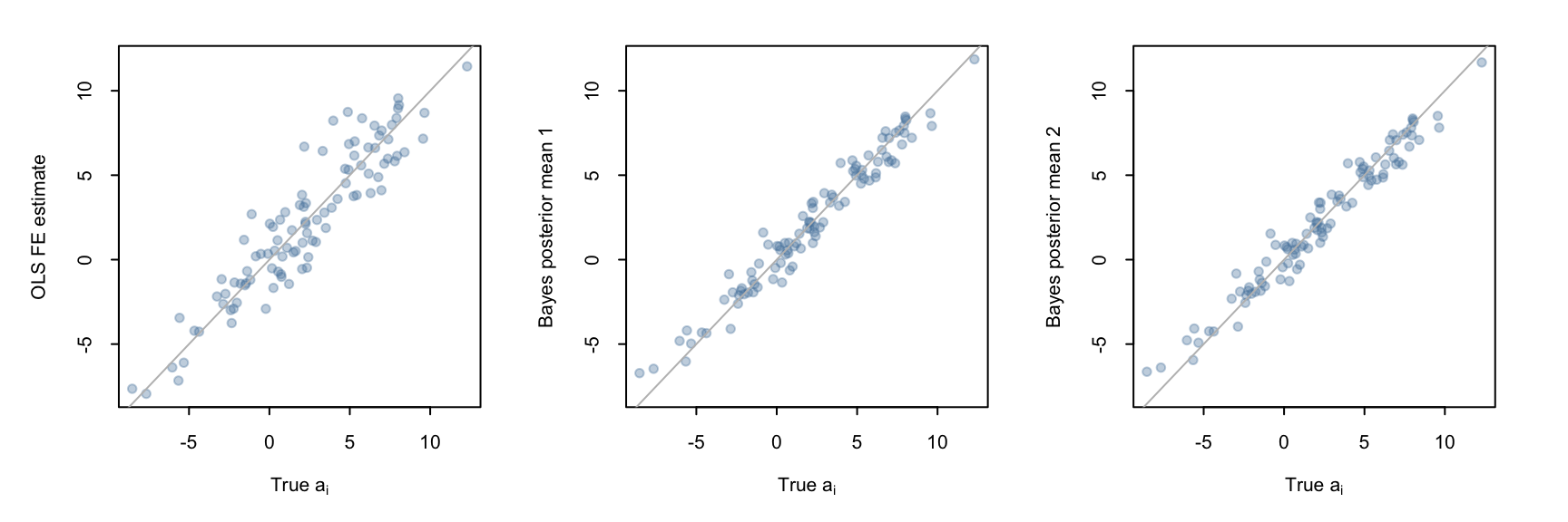

As we can see, the Bayesian estimates are less noisy than the OLS ones.

We can also see the same thing by comparing the differences between the $a_{i}$ estimates and the true firm mean values:

data.frame(
  bay1 = a_i_summary$mean - firm_mean,
  bay2 = a_i_summary2$mean - firm_mean,
  ols = fixef(olsfe)$firm_id - firm_mean
) |> 
summary()

      bay1                bay2                ols           
 Min.   :-1.732067   Min.   :-1.830365   Min.   :-2.858362  
 1st Qu.:-0.647746   1st Qu.:-0.728263   1st Qu.:-1.155375  
 Median : 0.022125   Median :-0.004072   Median :-0.008425  
 Mean   :-0.003507   Mean   :-0.028118   Mean   :-0.005805  
 3rd Qu.: 0.480510   3rd Qu.: 0.487135   3rd Qu.: 0.903697  
 Max.   : 2.447100   Max.   : 2.382485   Max.   : 4.523085